| Variable | Pre-Transformation Type | Post-Transformation Type | Purpose | Reason for Inclusion |
|---|---|---|---|---|
| review_star_rating | int | PCA scaled float | feature | literature survey |
| review_subjectivity | float | PCA scaled float | feature | literature survey |
| review_polarity | float | PCA scaled float | feature | literature survey |
| review_length | int | PCA scaled float | feature | literature survey |
| prod_subjectivity | float | PCA scaled float | feature | intuition |
| total_star_rating | float | PCA scaled float | feature | literature survey |
| site | dummy float | PCA scaled float | feature | intuition from EDA |
| review_helpful_votes | int | PCA scaled float | response | literature survey |
3 Models Implemented
In our modeling of the collected data, we seek to investigate several models for the generalization of the work performed by Guha Majumder, Dutta Gupta, and Paul (2022).
We will examine, compare, and contrast the use of the following models:
Multiple Linear Regression Prediction
Logistic Regression Classification
K-Nearest Neighbors Classification
Support Vector Machine Classification
3.1 Included Variables
3.2 Data Adjustments
As noted in our exploratory data analysis, each individual site has statistically significant differences in key variables we’re considering in our modeling. To mitigate the potential for under or overfitting, and misrepresentation due to variable scale we perform the following transformations to our data:
Variable outlier adjustment. We noted in our EDA that each of the e-commerce platforms had high volumes of outliers with respect to the inter-quartile range. We applied a transformation to our data to map any outlier variable value on a per-website basis from its value to \(\mu+3\cdot sd(\text{variable})\) for high-end outliers, and \(\mu-3\cdot sd(\text{variable})\) for low-end outliers. In the event that either of these values exceeded the minimum or maximum value of the dataset, we mapped the value to the minimum or maximum accordingly.
Standard scaling of variables. After adjusting outliers, we re-mapped all of our feature variables to be on the scale of the standard normal distribution \(N\sim(0,1)\)
Response variable transformation to binary value. We denoted a single useful vote as meaning that the review was useful to customers, and mapped the value to True/1, and False/0 otherwise.
Here is a sample (first 10 observations) of our data prior to the transformation:
| review_star_rating | review_subjectivity | review_polarity | review_length | prod_subjectivity | total_star_rating | site |
|---|---|---|---|---|---|---|
| 5 | 0.638000 | 0.461000 | 19.000000 | 0.350850 | 4.800000 | 1.000000 |
| 5 | 0.633333 | 0.211111 | 60.000000 | 0.617105 | 4.700000 | 0.666667 |
| 5 | 0.916667 | 0.787778 | 13.000000 | 0.480135 | 4.100000 | 1.000000 |
| 5 | 0.608333 | 0.266667 | 15.000000 | 0.658157 | 4.300000 | 0.666667 |
| 5 | 0.400000 | 0.180000 | 28.000000 | 0.658157 | 4.300000 | 0.666667 |
| 4 | 0.650000 | 0.433333 | 21.000000 | 0.617105 | 4.700000 | 0.666667 |
| 5 | 0.683333 | 0.300000 | 29.000000 | 0.350850 | 4.800000 | 1.000000 |
| 5 | 0.300000 | 0.750000 | 13.000000 | 0.460182 | 4.500000 | 1.000000 |
| 5 | 0.635417 | 0.516250 | 20.000000 | 0.350850 | 4.800000 | 1.000000 |
| 5 | 0.745887 | 0.470522 | 28.000000 | 0.435398 | 4.700000 | 0.666667 |
And here is a sample of our data after the applied transformations:
- Snippet of first 10 observations in our training dataset, post-transformation:
| review_star_rating | review_subjectivity | review_polarity | review_length | prod_subjectivity | total_star_rating | site |
|---|---|---|---|---|---|---|
| 0.527771 | 0.264387 | 0.336418 | -0.347482 | -1.353087 | 1.088999 | 0.722595 |
| 0.527771 | 0.240213 | -0.563168 | 0.998209 | 1.428196 | 0.716223 | -0.867221 |
| 0.527771 | 1.707921 | 1.512800 | -0.544412 | -0.002591 | -1.520431 | 0.722595 |
| 0.527771 | 0.110709 | -0.363171 | -0.478769 | 1.857024 | -0.774879 | -0.867221 |
| 0.527771 | -0.968488 | -0.675166 | -0.052086 | 1.857024 | -0.774879 | -0.867221 |
| -0.481349 | 0.326548 | 0.236820 | -0.281839 | 1.428196 | 0.716223 | -0.867221 |
| 0.527771 | 0.499220 | -0.243173 | -0.019265 | -1.353087 | 1.088999 | 0.722595 |
| 0.527771 | -1.486502 | 1.376802 | -0.544412 | -0.211017 | -0.029328 | 0.722595 |
| 0.527771 | 0.251005 | 0.535315 | -0.314660 | -1.353087 | 1.088999 | 0.722595 |
| 0.527771 | 0.823259 | 0.370697 | -0.052086 | -0.469912 | 0.716223 | -0.867221 |
Classes in the response variable (the number of helpful votes a review received) set were mapped as follows for all non-linear models:
0: if the review had no helful votes
1: if the review had one or more than 1 helpful votes
Our reasoning for this transformation is that, across the totality of our data, a comment receiving more than one vote as being useful is quite rare in our dataset, as uncovered during our exploratory data analysis. As such, even a single vote for being useful should put the comment in the running for being considered useful.
3.2.1 Dimensionality Reduction
For all models outside of the multiple linear regression, we performed a principal component analysis on the scaled data.
| Principal Component | Cumulative Variance | Explained Variance |
|---|---|---|
| PC1 | 0.350576 | 0.350576 |
| PC2 | 0.548099 | 0.197523 |
| PC3 | 0.673668 | 0.125569 |
| PC4 | 0.788246 | 0.114578 |
| PC5 | 0.878823 | 0.090576 |
| PC6 | 0.945954 | 0.067131 |
| PC7 | 1.000000 | 0.054046 |
To reduce dimensionality for Logistic Regression, Support Vector Machine, and K-Nearest Neighbor models, we elected to reduce from 7 principal commponents to 6. From the above table, we see that these 6 components explain approximately 95% of the variation within the training data. We projected our training and testing data from their 7-dimensional feature space to a reduced 6-dimensional principal component vector space and simplify computations. The only exception here is for our multiple linear regression, which used all 7 dimensions in its perscribed vector space.
3.2.2 Training Data
To train our dataset, we leveraged the data, post-transformation to train each of our models, including the adjustments of outlier datapoints to being within 3 standard deviations of the mean of each variable. We selected an 80% sample of this data and leveraged the same dataset to train each model.
In the interest of generalization, we sought to take our training dataset solely from products that were common across all three e-commerce platforms. By working with common data from each site, the data and the models may be able to formulate a more generalized construct of how certain variables behave within the different contexts of each platforms, and assist in better prediction and classification of comments as being useful or not.
3.2.3 Testing Data
For testing, we evaluated each model against transformed data, omitting the transformation of any outliers to being within 3 standard deviations of the mean. We performed this action to enable a fair comparison of each model against one another when working with real-world data.
3.2.4 Desired Outcomes and Objectives
Predictive modeling for the usefulness of a user comment on a product, in and of itself, cannot be conducted 100% objectively. We are interested in the exploration of misclassifications - particularly of false positives.
Our data exploration revealed that having even a single vote for a comment as being useful was exceedingly rare, with a median and mean number of votes hovering at or about 0 regardless of the website on which the comment was posted.
Additionally, from a technological perspective, the ability of a web user interface programmer or designer to simply filter or arrange comments by the number of votes they received is trivial.
With the above considerations in mind, we are interested in a model that provides reasonable accuracy while also having an apprpriate amount of recall and a reasonable F1 score. Having a model that perfectly maps predictions to actual outcomes is not useful to this research. Having a number of classified false positives for exploration and subjective evaluation is what interests us.
When exploring test results, we seek a percent of total positive predictions (true and false positives) matching that of the testing dataset. With this in mind, we won’t have the best accuracy, F1, precision, or recall. Having values for precision and recall hovering around 0.5 should support us in classifying reviews that have no votes as being useful as potentially being useful.
3.3 Examination of the Original Multiple Linear Regression
3.3.1 Linear Model Construction
We leveraged a similar formulation to that which was used within the research of Guha Majumder, Dutta Gupta, and Paul (2022).
Our version of the linear model is designed as follows: \(\hat{y} = \beta_0+\beta_1X_{rsr}+\beta_2X_{rs}+\beta_3X_{rp}+\beta_4X_{rl}+\beta_5X_{ps}\) \(+\beta_6X_{tsr}+\beta_7X_{s}\)
Where each of the following variables have been standard-scaled to a range between 0 and 1 for the input data:
\(X_{rsr}\) corresponds to the individual review’s star rating
\(X_{rs}\) corresponds to the review’s subjectivity score
\(X_{rp}\) corresponds to the review’s polarity score
\(X_{rl}\) corresponds to the review’s length (in words)
\(X_{ps}\) corresponds to the product description subjectivity score
\(X_{tsr}\) is the overall star rating for the product.
\(X_{s}\) is the site on which the comment was found (converted to a dummy variable for each website).
We leveraged \(X_{ps}\) as a proxy for the previous model’s binary attribute for whether or not a good was search-based or experienced based. Guha Majumder, Dutta Gupta, and Paul (2022) leveraged a set of binary variables to classify a good as being search, experience, or mixed products. Our intuition was that, given the subjectivity of a product’s description and/or specifications, a higher subjectivity score would correspond to an experience-based good, a lower subjectivity would correspond to a search-based good, and everything in-between would be a mixed product. This construction allows for any product to have a continuous potential range, and for most products to be mixed products (some tending more toward experience or search).
3.3.2 Inspection of Linear Model Assumptions
Generally, our examination of the multiple linear regression performed by Guha Majumder, Dutta Gupta, and Paul (2022) failed to meet the assumptions of linear regression (normality of residuals, linear pattern in fitted vs. observed values, and constant variance of residuals).
3.3.2.1 Linearity of the Model
Our model failed to achieve any clear form of linearity between fitted and observed values.
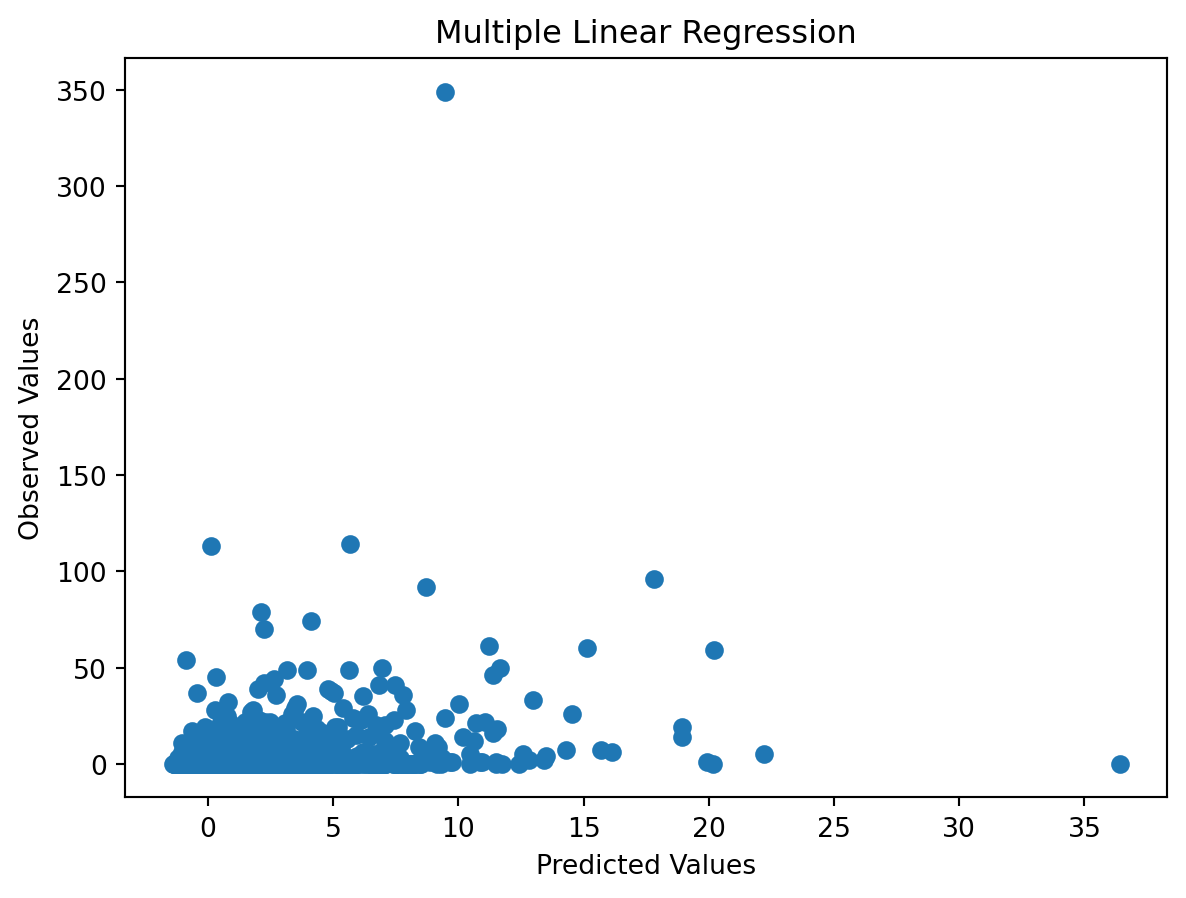
The fitted vs. observed values for this plot are not indicative of a linear pattern between the feature and response variables. It provides a high mean square prediction error of 28.4055, an \(R^2\) of 0.0884 and adjusted \(R^2\) value of 0.0883. The lack of even a moderate correlation here suggests one of the following:
The wider spread of data from multiple websites and wider range of products reduced the correlation found by Guha Majumder, Dutta Gupta, and Paul (2022)
The linear model is not generalizable.
The model is no better than randomly guessing the number of votes a comment could or should have associated with it.
What about if we filter down the testing data solely to reflect the positive cases - where the review comment has at least 1 vote for being useful?

The linearity issue remains even in this case.
3.3.2.2 Homoscedasticity on Normalized Data
This model has substantial challenges with heteroscedasticity. Let’s examine a plot of fitted vs. residuals in the model:

As expected for a model that does not have a clear linear pattern, the residuals for this linear model are heteroscedastic. We should expect to see a constant variance in a plot of predicted vs. residual values, with no correlation between the errors and the predictions. Here, we witness this issue directly, lending to the idea that the model is a poor fit for the data, and the nature of the model (e.g. additional data, additional features, or other feature/response transformations) would need to change substantially to produce effective predictive results.
3.3.2.3 Normality in Residuals
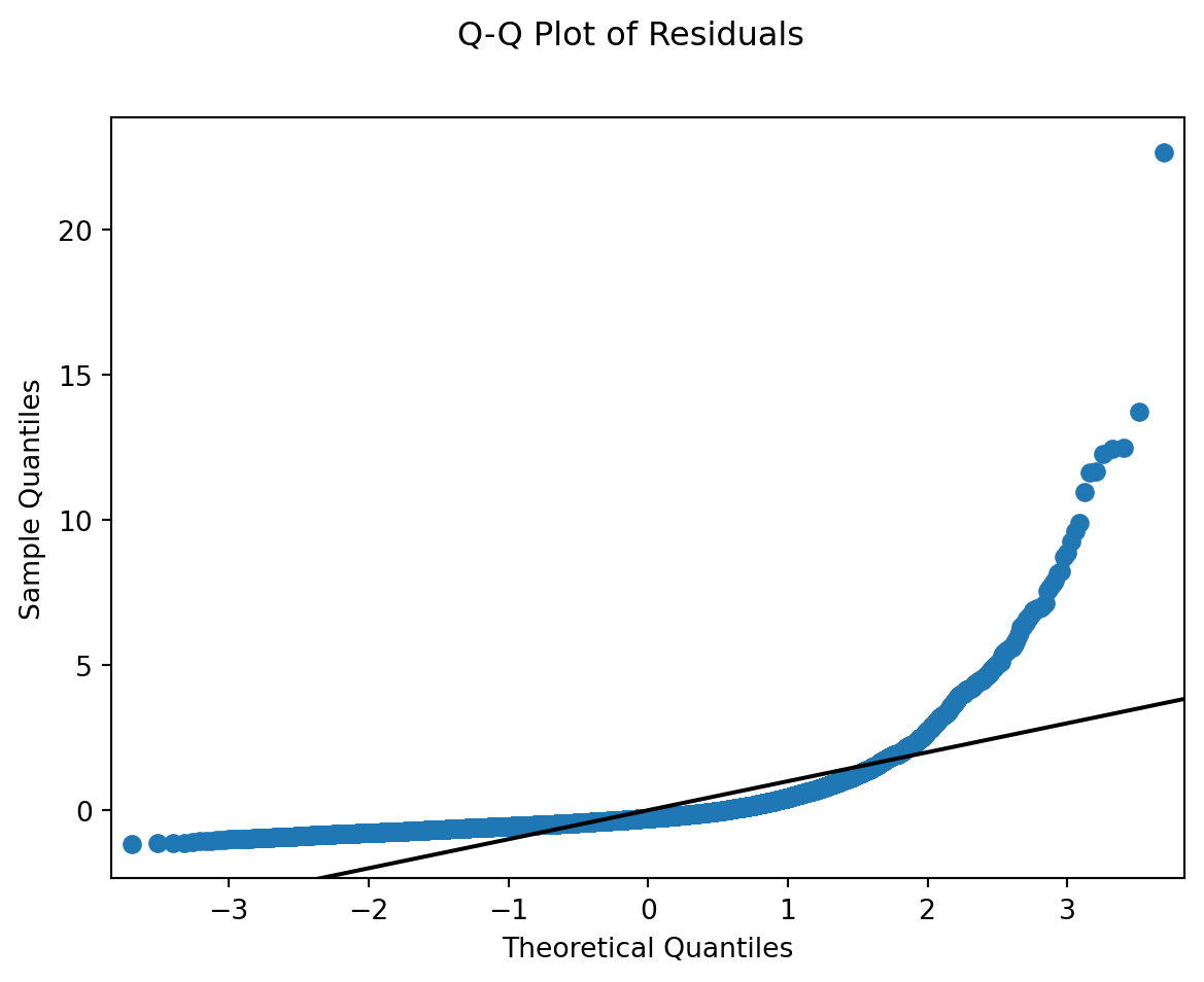
From the above plot, it is clear that this model fails to adhere to the multiple linear regression requirement for residual normality.
3.3.2.4 Conclusion on MLR model
Expanding the Multiple Linear Regression beyond the scope of the study performed by Guha Majumder, Dutta Gupta, and Paul (2022) seems to fail all of the assumptions of a linear model.
Irrespective of this finding, we will output the results of this model sorted in descending order of the score provided by the model, to compare and contrast with the findings of other models. A simple examination of the MLR with respect to its linearity may not be an effective means to evaluate this model’s performance.
Examining instead how the model predicts usefulness in comparison to other methods, alongside a subjective evaluation of the comments themselves may offer greater insight to its performance.
3.4 Logistic Regression Classification
Given the aforementioned challenges with the linear model, our next choice for examination was logistic regression. The MLR called for use of only numeric or continuous variables. Logisitic regression enables us to examine the inclusion of additional categorical variables as part of the regression consideration.
3.4.1 Hyperparameter Tuning
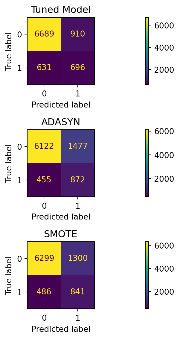
Logistic regression is, by our assessment, among the best performing models in our research effort. We inspected 3 logistic regression models - one tuned using the class weight hyperparameter to address the class imbalance present in the dataset. By assigning a higher weight to the minority class (1, or at least 1 vote for being useful) and a lower weight to the majority class (0, or no votes for the comment as being useful), the model was able to better capture the patterns associated with the minority class, leading to metrics in our target range.
3.4.2 Oversampling techniques
Additionally, 2 more logistic regression models are trained using two oversampling techniques, namely ADASYN and SMOTE. ADASYN, which generates synthetic samples for the minority class based on their difficulty in learning regions, and SMOTE, which creates synthetic samples by interpolating between existing minority class samples, were used to address the class imbalance problem. These techniques help to provide the model with more balanced training data, allowing it to learn the characteristics of both classes more effectively.
It is a well know fact that oversampling techniques can be employed in the event of a severe class imbalance if hyperparameter tuning does not improve the model performance. However, despite the heavy class imbalance, the tuned model and the SMOTE model achieve great result with approximately 80% accuracy indicating that it is proficient at making correct predictions. However, the models do differ in their scoring for precision and recall.
The tuned model delivers a higher precision and a lower recall, bouth around our target range of 0.4 to 0.55 for both, leaning us in the direction of examining the tuned model’s outputs for predicted useful comments. The “incorrect” prediction of elements from the minority class, which is what we’re looking for. We don’t want an over-prediction for false positives, but a reasonable degree of comments that could potentially be useful from a customer standpoint.
3.4.3 Logistic Regression Test Results
| Model | Accuracy | F1 | Precision | Recall |
|---|---|---|---|---|
| Logistic Regression (TUNED) | 0.827358 | 0.474599 | 0.433375 | 0.524491 |
| Logistic Regression (ADASYN) | 0.783554 | 0.474429 | 0.371222 | 0.657121 |
| Logistic Regression (SMOTE) | 0.799910 | 0.485006 | 0.392807 | 0.633760 |
Comments, sorted by probabability of being useful in descending order, are located here (link).
3.5 K-Nearest Neighbors Classification
K-Nearest Neighbors is used to learn and identify the target class instances. It makes predictions by calculating distance (usually, Euclidean distance) between a given instance and all other instances in the dataset in feature space.
3.5.1 Hyperparameter Tuning
The value of k is the most critial hyperparameter in the KNN Calssification algorithm. It determines the performance of the model. Usually a small k value leads to overly complex understanding of the data that might result into overfitting, however, a higher k values can lead to underfitting.
We have looked at multiple values of k for our given data and compared a set of model metrics - accuracy, F1 score, precision, and recall to find the most optimal model to be the model with k = 3.
As we did for our logisitc regression models, we leveraged the SMOTE oversampling technique to support each KNN model in better predicting true positive cases. Having additional co-located true-positive neighbors will impact the distance metric of test data points and the number of closest neighbors in a particular class.
3.5.2 KNN Test Results
Looking the results shown below we can say that:
KNN at each neighbor level performs poorer in comparison to logistic regression. The accuracy and precision do not reach sufficient levels. Furthermore, the total percent prediction of positive cases (ranging from 21.5-25.6%) far exceed the percent of true positive cases in the testing dataset (approximately 17%). These over-optimistic prediction levels (in combination with a high number of false negatives) suggest we may not be meeting the mark with this model, as once again, votes for a comment as being useful is relatively rare in this dataset.
For KNN with n=3 neighbors, we are the closest to the actual percent of positives in the source dataset. This model, however, has poor performance for precision, recall, and F1.
For KNN with n=9 neighbors, we improve the F1 score, but the precision and recall remain substantially low.
KNN, for any number of neighbors and given our selected features, may be an insufficient model for our use case. All of the KNN models far exceed our target % of total positive predictions. The source testing data has around 17% of the reviews as being “useful”, whereas each of these models’ positive predictions exceed that rate by at least 4%.
| Model | Accuracy | F1 | Precision | Recall |
|---|---|---|---|---|
| KNN (k=3) | 0.773807 | 0.372787 | 0.317125 | 0.452148 |
| KNN (k=5) | 0.771454 | 0.396450 | 0.326352 | 0.504898 |
| KNN (k=7) | 0.766973 | 0.408419 | 0.328004 | 0.541070 |
| KNN (k=9) | 0.762380 | 0.408698 | 0.324336 | 0.552374 |
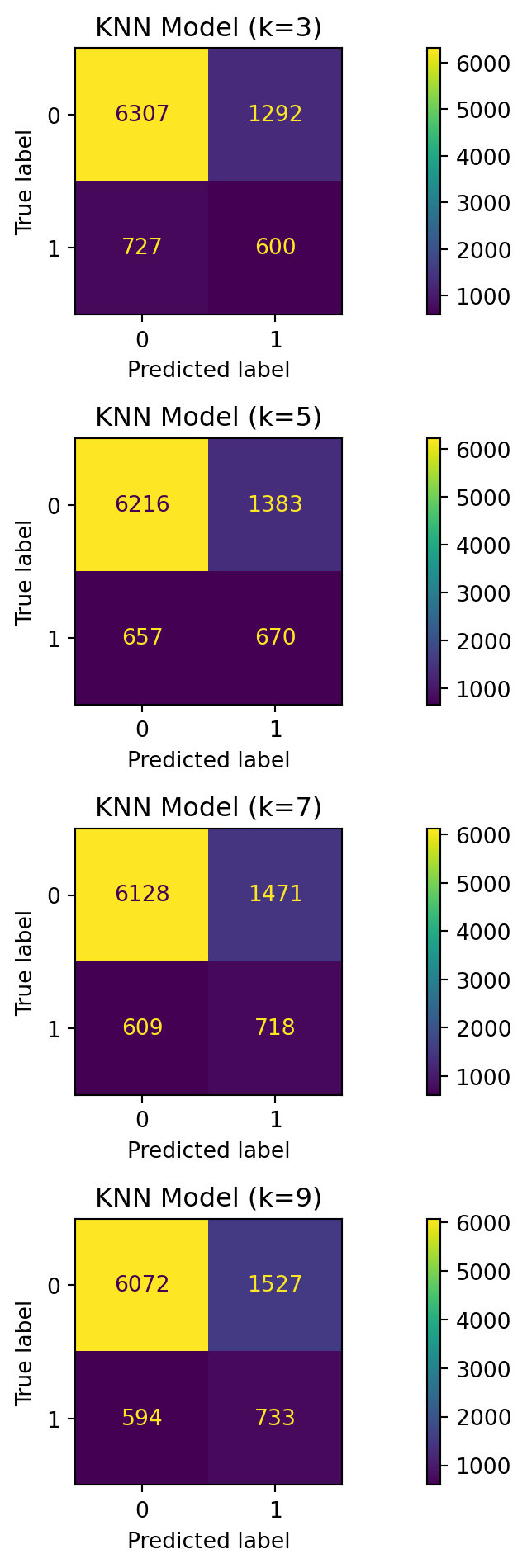
Simply examining the above confusion matrices, especially the upper-right hand corner false posistives, we see that KNN is likely over-optimistic about the usefulness of customer feedback. For the purpose of comparison to other models, we will examine the results of KNN n=3, as it held the closest value to the overall percent of true positives (17% true positives, 21.4% predicted).
3.6 Support Vector Machine Classification
Support Vector Machines work on classification problems by finding an optimal hyperplane that best classifies the target classes in the given feature space. Because of its flexibility of moving the hyperplane and adapting to the intricacies of the data, SVM could be a useful and powerful algorithm for our use case.
3.6.1 Hyperparameter Tuning
The complexity of a SVM model is determined by the choice of kernel function that supports the capturing of nuances within the data. Below are our implmentation results of the performance metrics of Support Vector Machine (SVM) models trained with different kernel functions: polynomial (SVM-Poly), radial basis function (SVM-RBF), and sigmoid (SVM-Sigmoid).
One note on our SVM-Poly implementation - it is equivalent to a standard SVM linear kernel, as we have implemented it with degree=1. We found during our evaluation, for reasons unknown to us, that polynomial implementation with degree 1 ran faster than that of the standard linear kernel. This was simply crafted this way to reduce execution time.
To tune each version of this model, we leveraged a reduced set of principal components, and adjusted class weighting, as having useful votes for a product is a relative rarity across each of the e-commerce platforms. To boost our recall, we elected to assign weights of 0.2 to class 0 (not useful) and 0.8 to class 1 (useful).
Furthermore, for the tuned model, we adjusted the probability threshold to 0.1 vs. the default 0.5 and class weighting set to better adjust the model for mis-classification of the minority class (as we did for the logistic regression). The combination of this shift with the class weighting allowed us to achieve a total positive prediction rate in close proximity to the actual true positives.
3.6.2 SVM Test Results
| Model | Accuracy | F1 | Precision | Recall |
|---|---|---|---|---|
| SVM-Poly | 0.827022 | 0.465374 | 0.430493 | 0.506405 |
| SVM-RBF | 0.849989 | 0.418079 | 0.493840 | 0.362472 |
| SVM-Sigmoid | 0.768205 | 0.367085 | 0.308960 | 0.452148 |
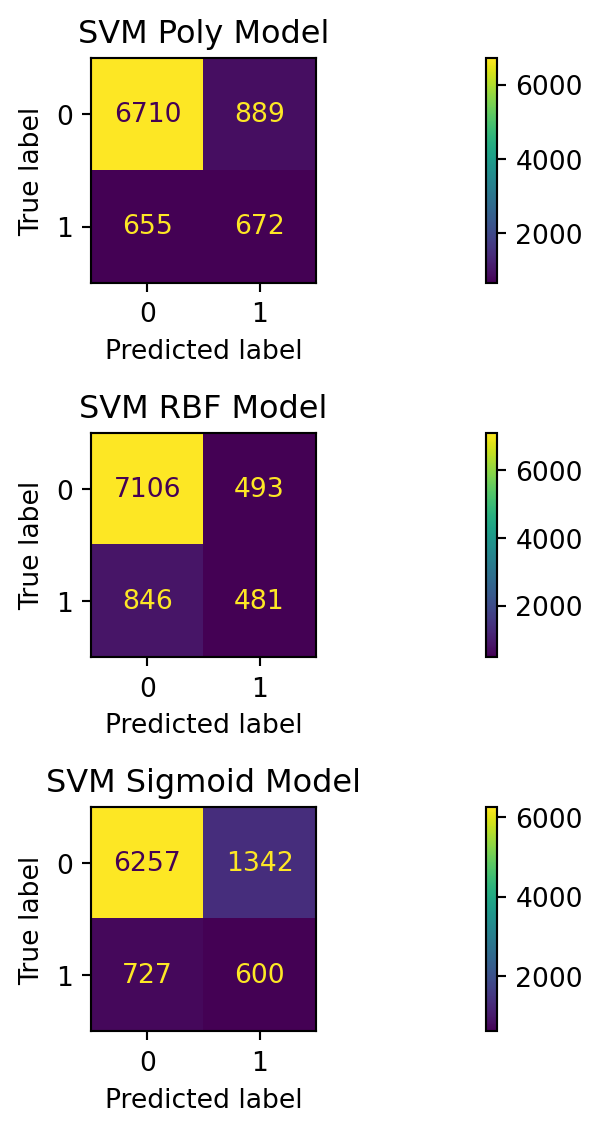
Looking the SVM testing results, we can say that:
SVM with a polynomial kernel (set to degree 1, or linear) predicts a total percent of true positives close to the underlying source data (approximately 17%).
SVM with radial basis function kernel appears to under-predict positive cases and fails to meet our F1 threshold.
SVM with sigmoid kernel over-predicts false positives and fails to meet our F1 threshold.
SVM Poly (linear, degree 1) appears to achieve reasonable accuracy while hitting an appropriate level for F1 and Recall for our use case. The presence of false positives gives us something to subjectively examine for its usefulness as a potential customer.
3.7 Model Comparison
We examine the following table to compare and contrast our implemented models on our collected data.
| Model | Accuracy | F1 | Precision | Recall |
|---|---|---|---|---|
| Logistic Regression (TUNED) | 0.827358 | 0.474599 | 0.433375 | 0.524491 |
| Logistic Regression (ADASYN) | 0.783554 | 0.474429 | 0.371222 | 0.657121 |
| Logistic Regression (SMOTE) | 0.799910 | 0.485006 | 0.392807 | 0.633760 |
| KNN (k=3) | 0.773807 | 0.372787 | 0.317125 | 0.452148 |
| KNN (k=5) | 0.771454 | 0.396450 | 0.326352 | 0.504898 |
| KNN (k=7) | 0.766973 | 0.408419 | 0.328004 | 0.541070 |
| KNN (k=9) | 0.762380 | 0.408698 | 0.324336 | 0.552374 |
| SVM-Poly | 0.827022 | 0.465374 | 0.430493 | 0.506405 |
| SVM-RBF | 0.849989 | 0.418079 | 0.493840 | 0.362472 |
| SVM-Sigmoid | 0.768205 | 0.367085 | 0.308960 | 0.452148 |
The most interesting results, we find, come from the tuned Logistic Regression model and SVM-Poly models. These seem to hit a sweet spot when it comes to F1 and recall scores. Exceeding certain thresholds (at or around 0.5), seems to have too high a percentage of false positives.
50% of our oversampled training data held votes as being useful comments, and our regular training data contained samples with approximately 7% being voted as useful.
For our testing data, approximately 17% of the records held votes for being useful.
The Tuned Logistic Regression predicted a total number of positive (true and false positives) of 1606, or 17.99% of the available samples. This result is very close in proximity to the actual total for true positives within the data.
The SVM Poly model also produced a prediction of approximately 17.5% of the testing data being useful (comparable to the actual value of 17%).
None of the other model formulations or permutations achieved a percentage of total positive prediction rate as in close proximity to the actual underlying data.
The false positives for SVM-Poly and Tuned Logistic Regression are located here:
For each of the models, the files are filtered to solely contain false positive reviews (those for which the model predicted the review is useful, but had no votes in favor of it in the source data).
Amongst the ranking of outputs from MLR, Logistic Regression, and SVM, we see some common threads.
Each recommended the same top 3 review comments for the following products:
Mario Kart 8 from Amazon.
Dyson Ball Vacuum from Target.
HP Deskjet 2755e Printer from Amazon.
| model | metric | review_subjectivity | review_polarity | review_star_rating | review_length | prod_subjectivity | total_star_rating | |
|---|---|---|---|---|---|---|---|---|
| 0 | Multiple Linear Reguression | mean | 0.515744 | 0.175872 | 4.100000 | 328.766667 | 0.481104 | 4.543333 |
| 1 | Multiple Linear Reguression | std | 0.084931 | 0.097946 | 1.268994 | 175.919786 | 0.071207 | 0.286095 |
| 2 | Logistic Regression (Tuned) | mean | 0.521513 | 0.108089 | 2.266667 | 258.933333 | 0.516312 | 3.940000 |
| 3 | Logistic Regression (Tuned) | std | 0.089206 | 0.135156 | 1.484014 | 211.463200 | 0.102916 | 1.164889 |
| 4 | SVM-Poly (Tuned) | mean | 0.515099 | 0.100752 | 2.066667 | 244.266667 | 0.513061 | 3.913333 |
| 5 | SVM-Poly (Tuned) | std | 0.083521 | 0.130734 | 1.412587 | 212.249192 | 0.101062 | 1.153027 |
Examining some metrics from the top 30 recommended “useful” reviews -
Logistic Regression and SVM had similar means and standard deviations for review star rating, review subjectivity, and review polarity. Each seemed to prefer slightly positive reviews (as follows from our EDA), and an even split on the subjectivity of the text (not overly precise, not overly vague). Similarly, they made more false positive predictions where the products subjective description of itself was near center, just like the review’s subjectivity.
Each model seemed to hold a preference for longer reviews, and for product descriptions that we assess may be considered “mixed” products (part search, part experience). Each model also held a bias for higher total star ratings for the product, with the MLR holding the greatest bias.
The MLR holds a bias toward higher star ratings (4.1) in its predictions. Similarly, it had a slightly greater bias toward positivity in the review. However, it held comparable results for subjectivity in comparison to SVM and Logisitic regression.
Generally the near “neutrality” with regards to polarity, subjectivity, and star rating for logistic regression and SVM could be useful to prospective customers. Allowing users to filter results based off of these predicted classifications could bring balance to other reviews presented when sorted in descending order by number of useful votes. The neutrality aspect can give the customer insight into unknown positive or negative reviews and shed light on useful information as a potential customer.
The presence of common reviews within the top 30 suggests that each of these models could hold a degree of validity. The interpretation and assessment, however, is subjective. Performing a further study with participants to evaluate the prediction of useful comments would support determining the validity of these models and their effectiveness.